Integrating Custom Trading Indicators with Pandas

On 18 February 2025 - tagged resources, python

Pandas has become the de facto standard for financial data analysis in Python. Its powerful data structures and efficient operations make it ideal for working with time series data. However, while pandas comes with many built-in functions, traders often need custom technical indicators for their analysis. In this post, we'll explore how to implement common trading indicators using NumPy and pandas in computationally efficient way and integrate them with Pandas dataframes seamlessly for convenience.

Let's start by defining a few utility functions that we'll use for efficient computation of the indicators:

Utility Functions #

Efficient Rolling Window Calculations #

When working with financial time series, we often need to calculate metrics over a rolling window of data. The naive approach of iterating through the data can be slow, especially with large datasets. Instead, we can use NumPy's stride tricks to create efficient rolling window views of our data:

def numpy_rolling_window(data, window):
    shape = data.shape[:-1] + (data.shape[-1] - window + 1, window)
    strides = data.strides + (data.strides[-1],)
    return np.lib.stride_tricks.as_strided(data, shape=shape, strides=strides)

The Decorator Pattern #

To make our indicator functions work seamlessly with both raw NumPy arrays and pandas Series, we use a decorator pattern:

def numpy_rolling_series(func):
    def func_wrapper(data, window, as_source=False):
        series = data.values if isinstance(data, pd.Series) else data

        new_series = np.empty(len(series)) * np.nan
        calculated = func(series, window)
        new_series[-len(calculated):] = calculated

        if as_source and isinstance(data, pd.Series):
            return pd.Series(index=data.index, data=new_series)

        return new_series
    return func_wrapper

This pattern allows us to write our core indicator logic using NumPy for performance, while still maintaining pandas compatibility.

Indicator Examples #

True Range #

The True Range indicator measures market volatility, taking into account gaps between periods:

def true_range(bars):
    return pd.DataFrame({
        "hl": bars['high'] - bars['low'],
        "hc": abs(bars['high'] - bars['close'].shift(1)),
        "lc": abs(bars['low'] - bars['close'].shift(1))
    }).max(axis=1)

Average True Range (ATR) #

The ATR is a moving average of the True Range, commonly used to measure market volatility:

def atr(bars, window=14):
    tr = true_range(bars)
    res = rolling_mean(tr, window)
    return pd.Series(res)

Relative Strength Index (RSI) #

The RSI is a momentum oscillator that measures the speed and change of price movements:

def rsi(series, window=14):
    deltas = np.diff(series)
    seed = deltas[:window + 1]

    ups = seed[seed > 0].sum() / window
    downs = -seed[seed < 0].sum() / window
    rsival = np.zeros_like(series)
    rsival[:window] = 100. - 100. / (1. + ups / downs)

    for i in range(window, len(series)):
        delta = deltas[i - 1]
        if delta > 0:
            upval = delta
            downval = 0
        else:
            upval = 0
            downval = -delta

        ups = (ups * (window - 1) + upval) / window
        downs = (downs * (window - 1.) + downval) / window
        rsival[i] = 100. - 100. / (1. + ups / downs)

    return pd.Series(index=series.index, data=rsival)

Bollinger Bands #

Bollinger Bands consist of a moving average and (usually) two standard deviation bands, used to identify overbought/oversold conditions:

def bollinger_bands(series, window=20, stds=2):
    ma = rolling_mean(series, window=window)
    std = rolling_std(series, window=window)
    upper = ma + std * stds
    lower = ma - std * stds

    return pd.DataFrame(index=series.index, data={
        'upper': upper,
        'mid': ma,
        'lower': lower
    })

Z-Score #

The Z-Score measures how many standard deviations a price is from its mean, useful for identifying extremes. Note that this implementation is not forward looking thanks to using rolling statistics!

def zscore(series, window=20, stds=1):
    std = numpy_rolling_std(series, window)
    mean = numpy_rolling_mean(series, window)
    return (series - mean) / (std * stds)

Pandas Integration #

To make our indicators easily accessible in pandas workflows, we can extend the PandasObject class:

from pandas.core.base import PandasObject

PandasObject.true_range = true_range
PandasObject.atr = atr
PandasObject.rsi = rsi
PandasObject.bollinger_bands = bollinger_bands
PandasObject.zscore = zscore

Now we can use these indicators directly on our DataFrame objects:

df['ATR'] = df.atr(window=14)
df['RSI'] = df.rsi(window=14)

Practical Example #

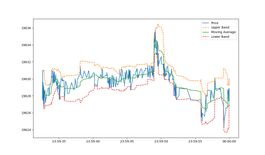
Let's apply these indicators to BTC prices from Crypto Lake free dataset:

import lakeapi
import matplotlib.pyplot as plt

# Get free sample data
lakeapi.use_sample_data(anonymous_access = True)
data = lakeapi.load_data(
    table = 'trades', 
    exchanges = ['BINANCE'], 
    symbols = ['BTC-USDT']
).set_index('origin_time')
data = data.iloc[-1000:] # Select just a few minutes of trades

# Calculate indicator
bands = data['price'].bollinger_bands(window=50)

# Plot results
plt.plot(data['price'], label='Price')
plt.plot(bands['upper'], label='Upper Band', linestyle='--')
plt.plot(bands['mid'], label='Moving Average')
plt.plot(bands['lower'], label='Lower Band', linestyle='--')
plt.legend()
plt.show()

Conclusion #

Full code in a single python file can be downloaded here. If you save the file, delete the usage in the bottom part and then import the module in your notebooks/analyses, you can build a convenient indicator library for your use-cases.

New posts are announced on twitter @jan_skoda or @crypto_lake_com, so follow us!